
There has been an ongoing discussion in the comments on previous posts about this problem, and it is also a problem often discussed in climate debate circles due to its importance in understanding how solar radiation reaches the Earth’s surface.
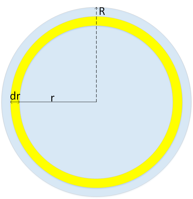
The problem in question is how one calculates the average projection factor of the incident solar radiation onto the hemisphere of the Earth which sunlight falls upon. To begin it might be helpful to look at the schematic of the cross-section of sunlight which is intercepted by the Earth:

The diagram above simply uses a factor of 0.5, which is what you get when you take a direct linear average by spreading the intercept-disk evenly over the hemisphere, and of course a hemisphere of the same radius has twice the area of a disk, hence the factor of 1/2 = 0.5.
However, the flux at any given location on the hemisphere is actually a function of the cosine of the solar zenith angle (with zero degrees pointing toward the sun, and 90 degrees toward the terminator at any azimuth), and, there is more surface area at larger zenith angles. Now, the cosine function spends more angular sweep between zero and ninety degrees above 0.5, while, there is increasing surface area above the angle where the cosine function equals 0.5. So we can only use calculus to see how these influences balance out. That is, to get the average projection, we must weight the projection with the surface area any particular projection value falls upon. So we need to do a weighted integrated average. We can exploit existing symmetry in this situation to make the integral more visual.
First, consider that for any given zenith angle the projection factor is the same, and hence, there will be bands about the hemisphere centered on the zenith axis which have the same projection factor. Consider that any given infinitesimal annulus on the input cross-section disk has a constant projection factor and falls onto a circular-section band of the hemisphere:
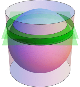
Each band of width dr falls onto a surface area of a hemisphere, and we should like to know how much surface area on a hemisphere that each dr occupies as dr goes to zero. For this, we exploit Archimedes’ Hat-Box Theorem:
-For any two parallel planes which cut off a band on a sphere, the surface area of the band on the sphere is the same as another band on a cylinder enclosing the sphere which is perpendicular to and cut off by the planes.
~or~
-For any two parallel planes with distance h between them which cut off a band on a sphere, the surface area of the band on the sphere is the same as the surface area of a cylinder band of height h with identical radius of that of the sphere.
A diagram with all necessary factors we’ll need is shown next:
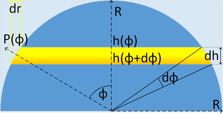
So what we need to do is integrate the projection factor multiplied by the weight for each projection factor “P”, and divide by the integral of the weights. The weights for each projection factor are of course the areas dA which they fall upon.
<P> = ∫P(φ)·dA(φ)dφ / ∫dA(φ)dφ
We should know what the integral of all band-area elements dA is already (the denominator above), given they all form a hemisphere, but we can write it out since the function is needed in the top of the equation multiplied by P(φ). Of course, P(φ) = cos(φ) where phi is the zenith angle.
The surface area of each infinitesimal spherical band annulus, dA, via Archimedes’ Hat-Box Theorem is
dA = 2πR·dh.
We want dA as a function of phi and hence dh as a function of phi, where dh is simply the difference in height along the zenith axis between h(φ) and h(φ + dφ), i.e.
dh(φ) = h(φ) – h(φ + dφ)
where h(φ) = R·cos(φ). Using the definition of an derivative, then
dh(φ) = -R·sin(φ)dφ.
That makes sense because dh is negative (h becomes smaller) when phi increases, and it changes only very slowly at first which is what the sin gives you. However, we only need the absolute value of dh since we are calculating area on the cylinder, which is positive. Hence
dA(φ) = 2πR²·sin(φ)dφ
Thus
A = ∫dA(φ)dφ = 2πR²·∫sin(φ)dφ where 0 <= φ <= π/2.
A = -2πR²·[cos(φ)] @φ = π/2 – @φ = 0
A = -2πR²·[0 – 1] = 2πR²
Of course we knew what that area was supposed to be, but we needed the differential form to use in the weighted integral. Thus
<P(φ)> = ∫P(φ)·dA(φ)dφ / 2πR²
= ∫cos(φ)·(2πR²)·sin(φ)dφ / 2πR²
= ∫cos(φ)sin(φ)dφ
= (1/2)·[sin²(φ)] @φ = π/2 – @φ = 0
= (1/2)·[1 – 0] = 1/2.
And so it turns out that the weighted integrated average projection factor on a hemisphere is the same as the simple linear average, even though the weighted projection function is not linear.
Now, the reason why we’re interested in the integrated average projection factor is because we can then multiply that by the top-of-atmosphere solar flux in order to get the integrated average flux on the input hemisphere. So that gives us the 1370 W/m² divided by 2, as we have in the top figure, and we can convert that to an equivalent forcing temperature as shown there too.
However, the relationship between flux and temperature is not linear but has a fourth-power exponential dependence between them, and so, the integrated average flux converted to temperature will not actually be the same as the integrated average flux when that flux is first converted to an equivalent temperature. The integrated average flux is certainly useful and interesting, but we are probably still more interested in the integrated average flux as converted to a temperature forcing. And so to calculate this we follow the same routine as above, but this time we first convert the flux “F” at each symmetric annulus band to a temperature via the Stefan-Boltzmann Law (T = (F/5.67e-8)1/4) and multiply that value with the weighting (as area) it falls upon.
<T> = ∫T(φ)·dA(φ)dφ / ∫dA(φ)dφ
= ∫ (F(φ)/5.67e-8)1/4·2πR²·sin(φ)dφ / 2πR²
= ∫sin(φ)·(1370·cos(φ)/5.67e-8)1/4dφ
= (1370/5.67e-8)1/4·∫sin(φ)·cos(φ)1/4dφ
= (1370/5.67e-8)1/4·(-4/5)·[cos(φ)5/4] @φ = π/2 – @φ = 0
= (-4/5)·(1370/5.67e-8)1/4·[0 – 1]
= (4/5)·(1370/5.67e-8)1/4
= (4/5)·394K = 315.2°K = 42.2°C.
If we want the value with the average absorptivity of 0.7 included, then we need to put the factor of 0.7 in with the flux to get
(4/5)·(0.7*1370/5.67e-8)1/4
= 288.5°K = 15.5°C.
This still isn’t really that meaningful of a number, because the rotating Earth spends quite a bit of angular sweep underneath input much closer to unity with the top-of-atmosphere flux, and it is this high-powered flux which creates cumulonimbus clouds, and the climate, etc.
The major point here of course being that it is 100% irrational, illogical, and incredibly stupid to average the incoming solar flux evenly over surface area it never exists upon, i.e. the entire surface area of the Earth at once, literally as if the Earth is a flat plane, etc.
New video up next soon, and it will be a doozy.

Brilliant!
http://m.wolframalpha.com/input/?i=%281361*0.7%2F5.67e-8%29%5E%281%2F4%29*%28integrate+sin%28x%29*%28cos%28x%29%29%5E%281%2F4%29+from+0+to+pi%2F2%29
Checks out!
That’s ~exactly US Standard Atmosphere global average.
Did you just figure this out, or is it in some document as well?
No I just wrote it out today.
One interesting incite that comes from the correct calculation is that we correctly see that the atmosphere cools the surface by 26.8°K, rather than the botton half of the atmosphere heating surface by 33°K (registered trademark of climate cult).
This makes perfect sense. If the atmosphere actually warmed the surface, the land/ocean would emit more atmosphere, which would emit more atmosphere, which would emit more atmosphere … until the earth became a giant gas ball like the sun, which would then heat the moon, until it too became a sun …
How do we still have solids in the universe?
I thought universe will die a heat death, but climate scientists claim everything goes to gas. Quite a stupid paradox.
/nerdy girl rant off
JP, TSI = 1370 is so retro. Are you trying to drive me nuts?
Sometimes the old fashioned things are the best.
JP,
You think 1370 is more accurate than 1361, on scientific grounds?
Or you don’t care enough to change an old habit?
“whatever” ?
Close enough.
The graphic is the one from your “The Model Atmosphere”
This result contradicts your “Absence of a Measurable Greenhouse Effect” diagram then
Zoe Phin…
Very interesting that the atmosphere cools the surface by 26º.8C.
There is an average increase of 3.3C/km in potential temperature with height due to a decrease in the adiabatic lapse rate in the presence of water vapour and its accompanying latent heat.
An 8km tropopause would give an increase in potential temperature of 26.4ºC at that altitude as result of evaporative cooling from the surface.
Thanks Joe. Brilliant as always! https://principia-scientific.org/how-to-calculate-the-average-projection-factor-onto-a-hemisphere/
Joe,
An absolutely facinating work of art in mathematics. I’m really really impressed !
As rosco pointed out, 0,637, which is 2/Pi, in the original diagram just changed to 0,5. How did you come up with 2/Pi in the first place. I still have to wrap my head over all of this.
Regards,
Yes I apologize for that Rosco. Originally when I first created that graphic I used the 0.5 factor because I had worked it out as such back then, and I worked it out simply numerically in Matlab with a big grid matrix. Then Alan produced his 2/pi result, and I thought that was pretty cool, so then I updated the graphic to use that figure and I figured maybe my numerical solution was wrong. I didn’t think anyone kept that updated graphic and I apparently forgot that I put it into a one of my publications. I thought it was not public anymore until I saw you post it here. Because after not-too-long I re-worked the problem and saw that the 2/pi solution wasn’t correct, and you can figure that because the geodesic lines on the hemisphere part from each other, rather than staying parallel as they do on the cylinder example. So then I changed the graphic back to 0.5 and it is the one I always use now for the past several years. And so, I thought that the question was finished, until it came up again here in the comments. I’ve been quiet on this because honestly I wanted to see what solutions people came up with, because hey maybe I was wrong. Finally, I decided to write out the solution formally and settle it once and for all, and hence this post. I’m sorry if has caused you to make arguments that are in the end incorrect. All of us here anyway understand what was being theorized, and *of course*, the correct value of the hemispheric factor is still not at all the main point, and it is still questionable whether this average number is all that meaningful given that the real point is that reality and physics occurs in *real time locally*, and hence the Sun has all the power required to create the climate and is *neither* a -18C input globally nor a +15C input hemispherically, etc.
Pierre, the 2/pi comes from integrating the cosine from 0 to pi/2, as an integrated average, to get the average projection factor over a 1-D cosine. Of course, the hemisphere is 2D and hence the solution in this post. But Alan Siddons (a Slayer from years ago) had presented an argument which made it seem like the hemispheric average projection should be the same as the 1-D cosine average. So it was like this:
= ∫P(φ)dφ / (φ2 – φ1) from φ1= 0 to φ2 = π/2
= ∫cos(φ)dφ / (φ2 – φ1) from φ1= 0 to φ2 = π/2
= [sin(φ)] / (φ2 – φ1) @φ2 = π/2 – @φ1 = 0
= [1 – 0]/(π/2 – 0)
= 1/ (π/2)
= 2/π
That is, the integrated average value of the cosine between 0 & π/2 is 2/π, which is larger than 0.5. Of course the range of the cosine in this sweep is between 1 and 0, but the average value of the cosine in this sweep is not simply the middle at 0.5, because the cosine spends more time above 0.5 than it does below it in the range 0 to π/2. The angle at which the cosine finally falls to 0.5 is of course acos(0.5) = 60 degrees, which is of course larger than 45 degrees (half the sweep between 0 and π/2).
Joe,
Thanks for the explanation. Please don’t sweat it. Science has always been 2 steps forward, 1 step back. It’s like climbing the proverbial wall of worries.
Still a wonderfull work of art in mathematics.
Regards,
Hi Joe,
Did the maths on the surface 0 to 23,5 degrees. I get 1368 * 0,15900 / 0,16588 = 1311 W/m^2. Allowing an albedo of 31% leaves us 905 for a mean temperature of 82C over that area
Did I get that right ? If so… Plenty of energy in day time to warm night time.
It’s likely close enough. But that point is indeed true. More energy is absorbed in day time than temperature which is actually generated. The balance is stored in latent heat of h2o and comes out at the poles and at night, etc.
Should you not take into account the refraction of sunlight towards the planet as it passes through the atmosphere? As such, we are receiving more than your model in which light travels in a straight line?
Interesting thought….might have a small effect around the terminator?
A good article although I think the geometry is presented in a more complex way than is necessary for the average reader. Once the Lambert cosine factor has been introduced the elemental area calculation should be more straight forward.
However, having said that, I can never understand why the earth’s albedo is claimed to be 0.7 while its emissivity is still taken as unity. Clouds form over warmed earth and reflect IR which is so very obvious on a warm cloudy night, as opposed to a clear night, scattering by aerosols of various sizes will, in general be similar for both visible and IR radiation. John Nicol (PhD Physics)
Yes IR readers do say in their manuals that they assume a 0.9 emissivity for example. It typically is material-dependant. The emissivity should likely at least be reduced to 0.9 or so.
… dh is negative (h becomes smaller) when phi increases …
h becomes smaller, as phi increases? — I’m confused [not surprising]
I’m seeing h becoming larger, as phi increases. Obviously, I need help.
It’s 6 minutes of extra sunlight, roughly a 1% increase. That’s important when your looking for your golf ball at 10:00 pm in June on the 47th parallel.
Well when accuracy to the 1% level is required…then for sure that’s important!!
Robert h is the height above the horizontal axis, dh is the band width.
I get the feeling your soul just needed to do this to prove to yourself that atmospheric physics does have more to it than showing a flashlight shining on sphere and explaining to your six year old daughter and scientists with PhDs in Climate science that the earth isn’t flat!
Geez I hate myself. I tried that 4-5 days ago and gave up because I did not like the answer. Talk about a reason.!?!?
Since the incidente surface of the Earth reduces as we go north or south as a function of COS(y)…
Double integrate from -Pi/2 to Pi/2
1368 * cos(x) * cos^2(y) dy dx
You get 1368 * Pi on the disk
On the hemisphere, 1368 * Pi / 2Pi = 1368 / 2
Is it just an accident ? Am I dreaming or is it true ?
I have taken a different approach to the study of CO2 induced global warming and climate change but come to the same conclusion. I would appreciate your comments on the exposition on my website at :
https://www.climateauditor.com
Fantastic Joseph !! .. just absolutely fantastic stuff !!! … BRAVO !!!
Greetings,
I have taken another approach to the CO2 induced global warming/climate change proposition at:
https://www.climateauditor.com
Any corrections, criticism or comments would be greatly appreciated as I think that we are both headed in the same direction.
Height above horizontal axis, duh, got it now. Thanks. For some reason, I was seeing h as the height of the respective triangle for which phi was its respective angle from 90 degrees zenith.
@wwf…yes I am either playing that video as dead pan…or my soul was dying a little. Seriously though…kindergarten for PhD’s! lol
Conclusion from Bevan’s link:
“The clear similarity between the autocorrelation function and the power spectra for the two time series, temperature and rate of change of CO2 concentration, from the Equatorial zone support the original contention that the temperature drives the rate of change of CO2 concentration. As the Tropics has the highest average temperature it must produce CO2 at the greatest rate. That CO2 must diffuse North and South away from the Equator into the Polar regions. As the solubility of CO2 increases with decreasing temperature it must be precipitated at the Poles within the ice and snow or as dry ice when the temperature is below its sublimation point of -78 degrees Celsius. That is, there may be a continuous circulation of carbon from the Equatorial Zone, through the atmosphere as CO2, to the Poles where it is locked into the Polar ice sheets until those sheets move sufficiently far from the Pole to melt. The CO2 is then concentrated in sea water and may return to the Equatorial zone via the Earth’s oceans.
That is, the Tropics is a source for the atmospheric CO2 and the Polar regions are a sink. As the seasonal variation from photosynthesis can be as great as 20 ppm in amplitude, it is possible that the almost 2 ppm per annum increase in CO2 concentration over the past 38 years has arisen from biogenetic sources driven by the natural rise in temperature following the last ice age. The Tropics has the greatest profusion of life forms throughout the Globe, so this may be a feasible source for the increase in CO2 concentration for that period. That could include an increase in the population of soil microbes thereby increasing the fertility of the soil leading to the greening of the Earth as can now be seen in satellite imagery. This is supported by an extensive study of global soil carbon which, quote: “provides strong empirical support for the idea that rising temperatures will stimulate the net loss of soil carbon to the atmosphere” end quote, Crowther et el 2016 [7].”
Cheers Squid!
I just watched the second half of the video again, and realized that I must have dozed off the first time I tried to watch it [no insult intended — I was tired at the time]. My reaction now: the video is wonderfully insulting, in the nicest, least aggressive, low-key way, to those who most needed it.
I’m loving this alternate Postma approach — what shall we call it? — “dead-pan/dead-soul approach” — most appropriate for the walking brain dead. (^_^)
My wife saw that I was running around the house…to the garage to get the light, upstairs to the play-area to get the globe, downstairs to the basement with it all. She was like “oh…I see what you’re doing. So…what are you doing?” I feel/felt like a FN idiot having to tell her. My reply that night was “Oh nothing…just a video”. The next morning she had been downstairs, and saw all the paraphernalia out. So she comes back up and asks, “So, how did the video go last night?” I said: “Well, it was a kindergarten demonstration like I do for [our daughter]…but for people with PhD’s.”
I mean…it just kinda makes my profession look FN retarded. And it makes my side-interest in this subject likewise. I mean…wives inevitably eventually lose all respect for their husbands…but, this just kinda hastens their resolve.
THAT’S HOW FN RETARDED THIS ALL THIS!!!!!!!!!!
But yah…that vid can be played as deadpan, but it is also taking a very soft approach towards adults who clearly lack the consciousness and mental subtlety to detect and distinguish very basic and simple things…like shadows. They would hence never see the deadpan. Maybe they need a soft guiding but serious hand, which is another way to take that vid. How you take that vid depends on your level of consciousness. Wickedwenchfan (and Robert and others of course) got it – high-consciousness individuals indeed!
Like I’ve written somewhere…the negative Hegelian dialectic and the increasing incorporation of cognitively-dissonant ideas among mainstream scientists has rendered them unconscious, or at least, has massively reduced their consciousness to the point that very simple things are beyond the degree of subtlety that their minds can comprehend. Their mental state has indeed become that of children, has become that of less-than kindergartners. They probably watch that vid in utter fascination, amazed at the pretty globe, and the bright shining light, etc. I mean, it must really F with them mentally and emotionally.
Hitler was a fan of deadpan. Uh oh.
The positive Hegelian dialectic is of course the increasing incorporation of cognitively-congruent concepts, and this produces higher levels of consciousness which can comprehend increasing degrees of subtlety.
It requires this higher level of consciousness to detect and enjoy deadpan.
This entire thing…this entire flat-Earth climate alarm edifice…is itself one of the greatest deadpan comedy routines of all time. And the butt of the joke, the object of the joke, is our scientific system and the people who practice it.
Bevan,
You may be interested in cloud cover changes.
There is 4 lines of convergent evidence that it’s the cause of the recent warming:
1) Cloud cover data since 1980s
2) Albedo changes since 1980s
3) Reduced relative humidity (contra AGW theory)
4) Increased outgoing longwave radiation (definitely contra AGW theory)
JP,
97% of scientists probably think you are a poo poo head for ruining their potty party.
That 97% act is if they are in the lowest 3% IQ. What they lack in intelligence they make up for in numbers.
If you add up all the IQs of the 97%, then you will get their average IQ, and I am sure that none of the higher-IQ members of this group would mind being characterized with an “average IQ” of such-and-such. After all, it this is basic math that they all agree on.
Joe,
I finally got to wrap my head around it. If you define what is happening on a hemisphere by using angle coordinates from -Pi/2 to Pi/2, N-S and E-W, and put these data on a plane, of course you will end up with a square plane. But the sum of all the points on this square plain is the sum of the points on the disk under the hemisphere. Using the right equation and dividing by 2Pi gives us back our mean on the hemisphere. Ouuufffff !!!!
So 1368 * cos(x) * cos^2(y) dy dx, correcting for less surface going away from the center, looks also to be a correct answer. 1368 / 2.
Tell me.
Regards,
Sorry Joe, I could have been more specific. I was referring to my page headed Greenhouse Effect and my Conclusion whereby there is far more energy arriving from the Sun in the CO2 absorption bands than is being emitted by the Earth’s surface. Thus far more of the Sun’s energy will be back-radiated into space than would be back-radiated by the atmosphere onto the Earth’s surface thereby causing cooling of the Earth not warming.
Ah I see. And yes, indeed!
Bevan and JP,
Take a look at Earth compared to Venus:
Hmmm, same CO2, different spectra!
Looks like the environment (temperature and pressure) sets CO2 absorption.
I’ll leave the conclusion for the wise to ponder. -Zoe
I’m still studying this, and I just want to make sure that I am clear: JP’s analysis disagrees with Alan Siddons’ analysis, right? If yes, then does the reason have to do with Alan’s not weighting properly his surface-area bands
Yes Robert, Alan’s reasoning did not take into account the increasing surface area a particular projection falls upon. There is increasing (annular) surface area with increasing zenith angle.
Robert,
Alan uses a 2D projection:
| -> (
Length of sun stick: 2R
Length of earth circle semi-circumference: PI*R
Ratio: 2/PI
What I did and what mainstream science does:
1361 × ∫ sin(φ) cos(φ) dφ (result = flux)
They get all the projections correct! But …
They don’t acknowledge holder’s inequality. Postma does.
That’s his key insight into this problem. It’s not his
projection math; those are the same:
(1361/5.67e-8)^1/4 × ∫ sin(φ) cos(φ)^1/4 dφ (result = temp.)
(The difference in the integral is the ^1/4)
Why is Postma’s way correct?
Because two same material and mass objects, one at 0°C, and one at 20°C will
come to an equilibrium of 10°C (a simple mathematical average)
But if we do this with fluxes:
10°C => 315.64 W/m^2
20°C => 418.74 W/m^2
AVG = 367.19 W/m^2 => 10.53°C
That is entirely incorrect.
Temperature is not set by averaging fluxes of 2 same objects.
Temperature is set by averaging temperatures of 2 same objects.
Is this something to do with Stefan-Boltzmann?
JP,
Unfortunately you will have to revise your statement that mainstream scientists moved the sun twice as far in light of your new math.
Let’s say F = 1361*0.7
Your math …
Temp = 4/5*F^0.25/sigma^0.25
Flux = Temp^4 * sigma
Flux = 256/625 * F (hemisphere)
Their math …
Flux = 1/2 * F (hemisphere)
Flux = 1/4 * F (sphere)
Ratios:
512/625 (hemisphere/hemisphere)
1024/625 (hemisphere/sphere)
They didn’t move the sun twice as far, they moved it 1024/625 = 63.8% farther.
Double check:
1361*0.7/4 = 238.17
http://m.wolframalpha.com/input/?i=%28%281361*0.7%2F5.67e-8%29%5E%281%2F4%29*%28integrate+sin%28x%29*%28cos%28x%29%29%5E%281%2F4%29+from+0+to+pi%2F2%29%29%5E4*5.67e-8
390.226 / 238.17 = 1.6384
It’s based on just looking at their TOA flux – their implied TOA flux. No need to covert that the temperature.
JP,
I disagree. Their TOA influx is the same. They pretend the outflux is the influx, but then you need the transformations.
If they moved the sun twice as far, then their calculations would be twice as wrong as their already 63.8% incorrect answer.
Zoe,
There is an other way. Correct the surface seen by the sun by cos(y) for going N or S….
F = 1368 * cos(x) * cos^2(y). Integrate that from -Pi/2 to Pi/2 for both integrals. You get 1368 * Pi. Since the hemisphere is 2Pi greater then a disk… 1368 * Pi / 2Pi = 1368 / 2.
Joe has not confirmed yet. It might be accidental but to me it looks perfectly OK.
JP,
No wait that didn’t make sense. They’re not 2x 63.8% wrong, but you get what I’m saying?
Falsification Of The Atmospheric CO2 Greenhouse Effects Within The Frame Of Physics by Gerlich & Tscheuschner pages 63 and 64 of the 2009 version. They cite Hölder’s inequality as to why the climate club derive the wrong expression.
This agrees with the expression Joe derives.
This publication caused such a storm of protest by the climate club the authors were effectively tried as witches – lucky they didn’t live in medieval times – they would have been burnt at the stake for “weather cooking”.
Pierre – if you want your head to explode read the Falsification … cited above or Proof of the Atmospheric Greenhouse Effect by Smith.
After acknowledging Hölder’s inequality it seems to me Smith just jumps right in using the factor 1/4 in a manner Gerhlich et al describe as inappropriate.
Smith does the default technique of restating the problem as if it’s the solution.
“Yes Robert, Alan’s reasoning did not take into account the increasing surface area a particular projection falls upon. There is increasing (annular) surface area with increasing zenith angle.”
I used to be good at this stuff but 3 decades of absence causes some incorrect assumptions that are hard to see – especially in 3D. I was happy with the 2D average resulting in 2/Pi and hoped it was another blunder for the climate club. The cosine of the angle of incidence from the zenith (or the “equator”) definitely gives the normal incidence at that point.
I copied Alan’s graphic
which appears to show an area factor.
As the normal is cos(φ) and the tangent is sin(φ) (the dr factor) the problem should have been as simple as the integral of cos(φ)sin(φ) dφ with the integral taking care of the details ?.
Yep for sure Rosco. I know I liked that result too, for the same reason. But still…mostly beside the point anyway.
“Smith does the default technique of restating the problem as if it’s the solution.”
I always said that was what Brown did with his ridiculous “proof” of the Steel Greenhouse. He just doubled the flux emitted by the shell and then used that to prove it emitted double the flux.
As you said at the time if the shell assumes the same temperature as Brown insisted then it would already be emitting the input flux of the sphere externally over a similar area so there was no reduction in flux emitted therefore no Steel greenhouse Effect. The shell of similar surface area to the inner sphere simply becomes the new emitting surface to space at the original flux – no need for perpetual motion.
Isn’t that amazing…that they just simply write it down, and draw it out, and then because they did that, doubling is OK and flat Earth is ok!? I mean…
I like that real truth seakers can admit to being swayed by someone’s seamingly correct arguments that later turned out to be wrong.
We can say “You got me; good one” and our opposition can’t. They can only double, triple, quadruple down on stupid. The conclusion must remain the same.
-Zoe
Rosco
“as simple as the integral of cos(φ)sin(φ) dφ with the integral taking care of the details ?”
I don’t see it. That integral from -Pi/2 to Pi/2 = 0 ! Or am I missing something ?
Rosco,
Forget about my last remark. I got it. You’re refering to Joe proof.
Sorry.
JP
The 1370W/m^2 TOA Solar Flux does that change by orbit/seasonal or not? Is the energy the exact same year around but the surface temperature variable? Sorry this is probably a freshman college question but I’m sure it will be argued by a climate clown at some point I just want to make sure I can explain it better if it comes up.
Earth’s orbit isn’t perfectly circular so it changes depending on position in orbit. I think it goes up to about 1410 W/m^2, and then likewise below 1370.
But its mainly the tilt that causes the season s of course.
My brother in law when he was working for the Air Force met a guy stationed in Australia whose job it was to “take the Sun’s temperature everyday” as he put it. Would be great to have that kind of information. I’ve seem sites that show the Sun and its spots etc but never TOA information. Convenient how they omit that from the data. Wouldn’t want anyone asking questions I guess.
JP and others…
Sticking with radiation then, I would be grateful for your thoughts on the shrinkage of the lapse rate in the presence of water vapour normally attributed to latent heat.
Moist air is a better radiator than dry so some energy must be radiated upwards to warm the cooler moist air at higher levels with a subsequent cooling of the lower warmer levels.
I wonder how much?
Pablo:
At section 1.2 of this paper
Click to access Absence_Measureable_Greenhouse_Effect.pdf
I show how to derive the lapse rate with water vapour latent heat release. The release of the latent heat in water vapour causes the slope of the lapse rate to lessen.
As for the surface, wet-areas at equal latitudes to dry-areas are generally cooler on average. This is due to the high heat capacity of H2O, which means it can absorb lots of heat without rising in temperature much…especially in the latent heat phase where it can absorb heat without increasing in temperature at all(!).
JP….
Thank you so much for the link.
The whole paper is brain fizzingly powerful…a new insight for me into the true power of latent heat.
There seems to be a growing interest in radiative absorption on other than flat earths. It is about time.
Dr. Charles R. Anderson recently posted a piece, in cooperation with Claes Johnson, that calculated the angular incidence of radiation on a sphere. https://objectivistindividualist.blogspot.com/2019/09/the-incidence-of-planar-radiation-upon.html. A slightly earlier consideration of absorption/emissions effects appeared in Prather, Michael J., and Juno C. Hsu, “A round Earth for climate models.” PNAS September 24, 2019 116 (39) 19330-19335; first published September 9, 2019 https://doi.org/10.1073/pnas.1908198116 .
Joseph, thank you for your wonderful post .”How to Calculate the Average Projection Factor onto a Hemisphere”Continuous Hemispherical System Input
= Fo (1-a)*0,5
= 303 K or +30
Do you consider Planet not only diffusely, but also specularly reflecting?
Cheers Christos. There’s both types I think. The oceans do a lot more specular.
Joseph, I am very glad to here that from you!!!
What I have found is that the planets’ satellite measured mean surface temperatures relate (everything else equals) according to their Rotational Spins the sixteenth root!
So I have a theory developed Planet Surface Rotational Warming Phenomenon..
But first about the two kinds of reflection:
When I realized that for the smooth planets surface the parallel solar rays irradiation should be not only diffusely reflected, but also specularly reflected, when I realized that I started searching for papers describing the solar parallel beams reflection from the spheres.
No matter how hard I searched for, there were none. So, I concluded there are not papers about the sphere’s the parallel solar beams specular reflection.
Since I could not let it there unsolved, I decided to look somewhere else.
I knew about the different shape bodies having different resistance to the liquid parallel flow when the Reynold’s Number is Re < 10000.
So I looked for a Table of Measured Drag Coefficients.
And, for a smooth sphere the Measured Drag Coefficient is
0,47
https://en.wikipedia.org/wiki/Drag_coefficient
I welcomed the 0,47 as the planet spherical surface solar irradiation accepting factor for the smooth surface planets without-atmosphere (an analogue of parallel liquid flow resistance).
Φ = 0,47 (Φ is from the Greek word Φως [phos], the light. Like in the Phosphorus.
And Φ varies from 0,47 for smooth surface without-atmosphere planets to 1 for heavy cratered planets, and 1 for gases planets.
0,47 ≤ Φ ≤ 1
Thus, solar system planets surfaces have been divided in three major categories – the smooth without atmosphere ones, the heavy cratered without atmosphere and the gaseous.
The heavy cratered planets and the gases planets do not reflect specularly, they reflect only diffusely.
During their multibillion years History, every planet has developed either a smooth surface Φ = 0,47 , or a heavy cratered Φ = 1.
Only Triton (Neptune’s satellite) does not get in either categories. In the case of the Triton Φ is neither 0,47 , no 1, but somewhere in between.
Energy in = energy out
Energy in = Φ(1-a)So πr^2 = 0,470,71361 πr^2 = 444 πr^2 ( W )
or, on average on the cross-section disk
Energy in = 444 πr^2 ( W ) / πr^2 ( m^2 ) = 444 W/m^2
and
the Energy out on average from the entire Earth’s surface
Energy out = 444 * πr^2 ( W ) /4 πr^2 = 111 W/m^2
Planet not only reflects diffusely Albedo a = 0,3
The diffusely reflected portion is 0,3*So
But Planet reflects specularly, and diffusely, and these two kinds of reflection do not summarize with each other, so the total reflected portion is:
(1 – 0,47 + 0,470,3)So πr^2 = (0,53 + 0,141)So πr^2 = 0,671So πr^2
The “absorbed” (not reflected), which is the emitted portion Is:
(1 – 0,671)So πr^2 = 0,329So πr^2 = 444 W/m^2 πr^2
Best regards,
Christos
At a first approach, when without the Rotational Warming phenomenon implementation, I use instead of Te, the Planet Corrected Effective Temperatures Te.correct
The formula is:
[ Φ(1-a) /4σ ]^1/4
Φ = 0,47 (the 0,47 is for smooth surface planets without atmosphere, the factor Φ accounts for the smooth planet surface specular reflection)
Table of results for Te and Te.corrected
Planet…….. Te……….Te.correct
Mercury…..440 K…….364 K
Moon………270 K……224 K
Earth………255 K…….210 K
Mars,,,,,,,,,,210 K……174 K
Yes, Joseph. The oceans do a lot more specular.
Joseph,
A question about the 70 % average absorption, which gives in your calculation:
4/5 ∜((0.7×1370)/(5.67×10^(-8))) = 288. 5 kelvin
Shouldn’t we fill in 50 % absorption in the earth’s surface (and 20 % absorbed in the atmosphere)?
4/5 ∜((0.5×1360)/(5.67×10^(-8))) = 265 kelvin
This outcome (average surface temperature) would require a natural greenhouse effect to explain the 288 K!
Johan (electrical engineer)
@Johan: that calculation is for the whole Earth system, and so it uses the albedo for the whole system, which gets you the total energy output for the whole system, which then gets you the effective temperature for the entire integrated system, surface + atmosphere, etc.
See here:
So, you get 255K (-18C) for the effective temperature. This temperature by definition could only be found around the average of the system, and the average of the system is not the slice of air closest to the ground. The slice of air closest to the ground must be warmer than the expected average, due to he adiabatic gradient, and due to the fact that the initial solar heating takes place at the ground, i.e., at the slice of air closest to the ground. So, the average temperature must be found at altitude. If you go to where it is found, -18C at 5km altitude, then the adiabatic gradient alone explains why the surface slice of air is 288K. If there were a radiative greenhouse effect, then the calculation wouldn’t work, because the adiabatic gradient would be modified to a different slope than what the adiabatic calculation directly gives you.
Ok, thanks for your clarification.
Would your calculation method also apply to planet Venus with an optically thick atmosphere and planet Mars with an optically thin atmosphere? Checking whether or not your weighted integrated average temperature calculations approach NASA’s fact-sheets, https://nssdc.gsfc.nasa.gov/planetary/factsheet/ ?
Regards, Johan (EE)
This method is standard practice, as all that it requires is the albedo of the planet. The albedo factors everything in.
Yes it works anywhere.
Joseph, I filled in the relevant values in your formulae for the Moon, Venus and Mars and I found huge discrepancies compared with NASA’s fact sheet on the average temperatures:
Earth Moon Mars Venus Sun
Radius [m] 6.37E+6 1.74E+6 3.40E+6 6.05E+6 696E+6 Distance from Sun [m] 150E+9 150E+9 228E+9 108E+9 –
Planet-Sun view factor 2.16E-5 2.16E-5 9.32E-6 4.14E-5 –
Bond albedo 0.30 0.12 0.25 0.77 –
Power density [W/m^2] 62.8E+6
Solar irradiance [W/m^2] 1360 1360 586 2600
Emission temperature [K] 255 270 210 227 5770
Calculated average Ts [K] 288 305 237 256
Fact Sheet NASA [K] 288 253 208 737
Stefan-Boltzmann constant σ = 5.67E-08 [W/(m^2 K^4)]
I’m afraid there’s a problem with this algorithm after all. Possible reasons:
– No heat retention on Moon and Mars by liquid H2O.
– Heating on Venus by atmospheric pressure (92 bar) and/or by spinning retrograde.
to be cont’d?
The NASA fact sheet just does it with the albedo method, so it should work. Unless they’re reporting surface temperature, which is different than effective temperature. For effective temperature you would go:
Teff = ((R_Sun/D_planet)^2 * T_Sun^4 * (1 – albedo) / 4)^(1/4)
T_Sun = 5778K
R_Sun = 695,700,000 (meters)
D_planet = distance of planet from Sun (meters)
If they’re reporting surface temperature then that is different, and you need to apply the adiabatic gradient for the specific planet’s atmosphere. This is what Nikolov & Zeller have shown. Basically you find either the average atmosphere location, or the altitude at which it has Earth’s surface pressure & temperature, and then apply the adiabatic gradient from there.
Your values aren’t far off so I think maybe there was just a typo in your equation, or you’re reading surface temperature instead of effective temperature from the fact sheet.
@ Joseph, yes indeed, I interpreted NASA’s fact sheet values wrongly regarding mean or effective versus surface temperature.
Unfortunately my “table” formatted with blanks went wrong 😦
Earth Moon Mars Venus
Distance from Sun [m] 150E+9 150E+9 228E+9 108E+9